Introduction
Metis Bootcamp Project 1
Collaborators: Dean Miao, Derek Shi and Joseph Hamilton.
This will be the first of several Metis Bootcamp projects.
The Problem
WomenTechWomenYes was hosting their annual gala at the beginning of summer and wished to increase the number of attendees (and possible donors) by standing outside of New York City Subway Stations and letting people sign-up to collect free gala tickets through email.
My Approach
Our goal for the project was to find the stations with the highest traffic data from the MTA website. While the data was easy to obtain, it contained a significant amount of errors. To reduce the number of errors that incur while cleaning data, I chose to use a weighted average method. As with most cleaning methods, a reduction error comes with an increase in processing power. The Weighted Average Method explained in this post is more complicated than the method introduced by Joseph Hamilton but will give more accurate results. In a later post I will compare the two methods to see how the final results compare to the computational power needed to obtain those results (i.e. was it worth the pain).
The Data
Introduction
When first obtaining the data set from the MTA website the following variables are given:
| Variable | Description |
|---|---|
| C/A | Control Area name/Booth name. This is the internal identification of a booth at a given station. |
| UNIT | Remote unit ID of station |
| SCP | Subunit/Channel/position represents a specific address for a given terminal in each unit. |
| STATION | Subway Station name. |
| LINENAME | Train lines stopping at this location. |
| DIVISION | Represents the Line originally the station belonged to. |
| DATE | Represents the date of the audit data (MM/DD/YYYY). |
| TIME | Represents the time of the reported data (HH:MM:SS). |
| DESC | Represents the if scheduled audit event went normally. |
| ENTRIES | The cumulative entry register value for a device. |
| EXITS | The cumulative exits register value for a device. |
Using a pandas dataframe we can see an example of the output of the table.
| C/A | UNIT | SCP | STATION | LINENAME | DIVISION | DATE | TIME | DESC | ENTRIES | EXITS | |
|---|---|---|---|---|---|---|---|---|---|---|---|
| 0 | A002 | R051 | 02-00-00 | 59 ST | NQR456W | BMT | 02/18/2017 | 03:00:00 | REGULAR | 6055520 | 2052786 |
| 1 | A002 | R051 | 02-00-00 | 59 ST | NQR456W | BMT | 02/18/2017 | 07:00:00 | REGULAR | 6055537 | 2052800 |
| 2 | A002 | R051 | 02-00-00 | 59 ST | NQR456W | BMT | 02/18/2017 | 11:00:00 | REGULAR | 6055600 | 2052891 |
| 3 | A002 | R051 | 02-00-00 | 59 ST | NQR456W | BMT | 02/18/2017 | 15:00:00 | REGULAR | 6055822 | 2052960 |
| 4 | A002 | R051 | 02-00-00 | 59 ST | NQR456W | BMT | 02/18/2017 | 19:00:00 | REGULAR | 6056158 | 2053035 |
To begin with, the easiest variables to throw out are LINENAME, DIVISION and DESC. Since we are looking for ridership for each station, the variables representing the lines that connect the stations or the original Line that owned the station are not needed for the analysis. Furthermore, the variable DESC is not needed because we will adjust for irregular time intervals within The Weighted Average Method. The goal now is to find the unique identifier for each turnstile in each station.
Unique Turnstile Identifiers
Every individual turnstile in the MTA system has a unique identifier that can be found using a combination of booth name, unit ID, SCP and station. Finding erroneous variables in the unique turnstile identifiers requires combining the variables C/A, UNIT, and SCP and finding the number of unique values. Note, the data will be later split by station, so it does not need to be included in the unique identifier.
| Possible Turnstile Identifiers | Number of Unique Identifiers |
|---|---|
| C/A UNIT SCP | 4732 |
| UNIT SCP | 4732 |
With the number of unique identifiers being equal for both identifiers and the definition of the variable C/A it is clear that the variable C/A is not needed. In additional prework, it also became apparent that there are more unique units than stations. Using this information, it is appropriate to assume that there are individual sations that have more than one unit.
| Variable | Number of Unique Values |
|---|---|
| UNIT | 468 |
| STATION | 378 |
Furthermore, by a visual inspection it was apparent there are examples of non-unique SCP values for an individual unit; hence, both variables are needed to create a unique identifier for a turnstile in a given station. With this in mind, the final variables used in the analysis will be UNIT_AND_SCP (a combination of unit and SCP), STATION, DATE_AND_TIME (a combination of the date and time to create one time point), ENTRIES and EXITS.
| UNIT_AND_SCP | STATION | DATE_AND_TIME | ENTRIES | EXITS | |
|---|---|---|---|---|---|
| 0 | R051 02-00-00 | 59 ST | 2017-02-18 03:00:00 | 6055520 | 2052786 |
| 1 | R051 02-00-00 | 59 ST | 2017-02-18 07:00:00 | 6055537 | 2052800 |
| 2 | R051 02-00-00 | 59 ST | 2017-02-18 11:00:00 | 6055600 | 2052891 |
| 3 | R051 02-00-00 | 59 ST | 2017-02-18 15:00:00 | 6055822 | 2052960 |
| 4 | R051 02-00-00 | 59 ST | 2017-02-18 19:00:00 | 6056158 | 2053035 |
Creating Station Specific Tables
Once narrowing down to only the necessary variables, the data can now be separated by individual station entries and individual station exits. This information will be placed in a dictionary where the key is a combination of the station name and if the data points are for entries or exits and the value is a dataframe with the date and time variable for the index values, and the columns holding the cumulative data for either the entries or exits for each turnstile. For example, the following table is a part of the table for key 59 ST ENTRIES.
| UNIT_AND_SCP | R050 00-00-00 | R050 00-00-01 | R050 00-00-02 | R050 00-00-03 | … |
|---|---|---|---|---|---|
| DATE_AND_TIME | |||||
| 2017-02-18 03:00:00 | 6240218.0 | 8456367.0 | 2810319.0 | 52911.0 | … |
| 2017-02-18 07:00:00 | 6240237.0 | 8456370.0 | 2810321.0 | 52912.0 | … |
| 2017-02-18 11:00:00 | 6240273.0 | 8456398.0 | 2810328.0 | 52917.0 | … |
| 2017-02-18 15:00:00 | 6240409.0 | 8456484.0 | 2810371.0 | 52929.0 | … |
| 2017-02-18 19:00:00 | 6240650.0 | 8456654.0 | 2810441.0 | 52954.0 | … |
The Weighted Average Method
What is a Weighted Average?
What is a weighted average and how is it different from the standard average? The definition of a weighted average for a set of \(n\) numbers, \(x_1, x_2, \ldots, x_n\) is
where \(w_k\) denotes the weight for the \(k^{th}\) element in the data set. The weights picked can be any non-negative number (\(w_k\geq 0\)) for all \(k\) with the caveat that
When referencing the standard average of a set of \(n\) numbers, \(x_1, x_2, \ldots, x_n\) is
Notice the similarities in the equations for \(\bar x\) and \(\bar x_w\). The difference is that for a weighted average the individual data points are being multiplied by \(w_k\) and in the standard average they are being multiplied by \(1/n\). Now notice adding \(1/n\) \(n\) times will yield 1,
which satisfies the conditions for the weights in the weighted average. Hence, the standard average is a weighted average with equal weights on each point.
Why Use a Weighted Average?
A weighted average is used in finding an estimate for a set of data points where it is known that some data points are a better representation of the desired estimate. For example, consider a class with unknown number of students. On the first exam there are two possible grades to earn: 50 and 100. If asked about the expected average grade for the class, the best point with the information given is the standard average:
To the best of our knowledge, there is an equally likely chance a student will earn either a 50 or 100; therefore, the weights should be equal. Now, if it was known that \(90\%\) of the past students scored a 100, then a better estimate for the expected average grade would be:
Notice that the weights \(0.90\) and \(0.10\) satisfy the criteria of adding to one. While, which weights to choose are not always clear, for our problem it is.
Ridership Problem
Theoretically, each individual turnstile in each station recorded a cumulative count for entries and exits for every four hours starting at time 00:00 (midnight); however, in practice, approximately 52% of the data set contains times that did not fall on these time points. For each time point that does not fall on the desired time points there will be data for a time that is earlier (left time) and later (right time) than this time. For example, if there is not a data point for 08:00 but there are data points at 05:00 and 09:00.
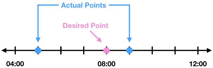
The data point at 09:00 is only one hour from 08:00, whereas the data point at 05:00 is 3 hours from 08:00.
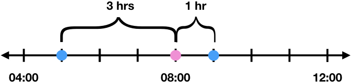
Because of this, the actual data for 08:00 should look more like the data point for the closer time, 09:00. Therefore, the weights for the weighted average should depend on the amount of time between the desired time point and the higher and lower time points. Since the distance from the desired time point and how important the data point is are inversely related, a good starting place for the weights are the inverse of the distance.
| Notation For Weight | Time Points | Distance from Desired Time Point | Initial Weight Guess | |
|---|---|---|---|---|
| High Time Point | \(w_r\) | 09:00 | 1hr | \(1/1=1\) |
| Low Time Point | \(w_l\) | 05:00 | 3hrs | \(1/3\) |
While a weight of 1 will but more emphasis on the data point for 09:00 compared with a weight of 1/3 for 05:00, the sum of the weights do not equal one. Fixing this will require normalizing the weights with a normalizing constant, \(N\).
From the above equations, it is apparent the normalizing constant is the sum of the two distances. Using the normalizing constant of 4/3 in the above table will give us the appropriate weights for the weighted average.
| Notation For Weight | Time Points | Distance from Desired Time Point | Initial Weight Guess | Normalizing Constant | Actual Weights | |
|---|---|---|---|---|---|---|
| High Time Point | \(w_r\) | 09:00 | 1hr | 1 | 4/3 | \(\displaystyle \frac{1}{4/3}=\frac{3}{4}\) |
| Low Time Point | \(w_l\) | 05:00 | 3hrs | 1/3 | 4/3 | \(\displaystyle \frac{1/3}{4/3}=\frac{1}{3}\) |
To expand this to a more generalized example we will denote the following variables:
| Time Point Variables | Time Point Descriptions | Cumulative Ridership Variables | Cumulative Ridership (Data Point) Description |
|---|---|---|---|
| \(x\) | Desired time point | \(\bar c_w\) | Cumulative ridership for the desired time point |
| \(x_r\) | Time point above (to the right) of the desired time point | \(c_r\) | Cumulative ridership for the time point above (to the right) of the desired time point |
| \(x_l\) | Time point below (to the left) of the desired time point | \(c_l\) | Cumulative ridership for the time point below (to the left) of the desired time point |
Generalizing the example using the above notation we have:
| Notation For Weight | Time Points | Distance from Desired Time Point | Initial Weight Guess | Normalizing Constant | Actual Weights | |
|---|---|---|---|---|---|---|
| High Time Point | \(w_r\) | \(x_r\) | \(x_r-x\) | \(\displaystyle \frac{1}{x_r-x}\) | \(\displaystyle \frac{1}{x_r-x}+\frac{1}{x-x_l}\) | \(\displaystyle \frac{\frac{1}{x_r-x}}{\frac{1}{x-x_l}+\frac{1}{x_r-x}}=\frac{x-x_r}{x_l-x_r}\) |
| Low Time Point | \(w_l\) | \(x_l\) | \(x-x_l\) | \(\displaystyle \frac{1}{x-x_l}\) | \(\displaystyle \frac{1}{x_r-x}+\frac{1}{x-x_l}\) | \(\displaystyle \frac{\frac{1}{x-x_l}}{\frac{1}{x-x_l}+\frac{1}{x_r-x}}=\frac{x_r-x}{x_l-x_r}\) |
Hence the weighted average using the length of time as weights is given by:
How Does This Look in Python?
In Python I was able to create a code that resampled the time points into the desired four hour intervals and found the weighted averages for each turnstile using pandas. Unfortunately, the function I created was only able to do this for one turnstile at a time (the computationally heavy downside).
Remember the table we last left off with?
| UNIT_AND_SCP | R050 00-00-00 | R050 00-00-01 | R050 00-00-02 | R050 00-00-03 | … |
|---|---|---|---|---|---|
| DATE_AND_TIME | |||||
| 2017-02-18 03:00:00 | 6240218.0 | 8456367.0 | 2810319.0 | 52911.0 | … |
| 2017-02-18 07:00:00 | 6240237.0 | 8456370.0 | 2810321.0 | 52912.0 | … |
| 2017-02-18 11:00:00 | 6240273.0 | 8456398.0 | 2810328.0 | 52917.0 | … |
| 2017-02-18 15:00:00 | 6240409.0 | 8456484.0 | 2810371.0 | 52929.0 | … |
| 2017-02-18 19:00:00 | 6240650.0 | 8456654.0 | 2810441.0 | 52954.0 | … |
Each turnstile would be sent into the weighted_average function and called df. To prepare for the weighted average the column would be renamed Number and the Date and Time would be added as a column to keep the values for finding the weights. For the turnstile R050 00-00-00 this looks like the following:
| Number | Date | |
|---|---|---|
| DATE_AND_TIME | ||
| 2017-02-18 03:00:00 | 6240218.0 | 2017-02-18 03:00:00 |
| 2017-02-18 07:00:00 | 6240237.0 | 2017-02-18 07:00:00 |
| 2017-02-18 11:00:00 | 6240273.0 | 2017-02-18 11:00:00 |
| 2017-02-18 15:00:00 | 6240409.0 | 2017-02-18 15:00:00 |
| 2017-02-18 19:00:00 | 6240650.0 | 2017-02-18 19:00:00 |
The left time and data point were obtained using resample and the resample function first. The label was taken to be the left number of the four hour sample bin and the interval would be closed on the left number.
df_L = df.resample('4H',label='left',closed='left').first()
df_L = df_L.rename(columns={'Date':'Right_Date','Number':'Right_Number'})
For example, the time interval from 04:00 to 08:00 would be represented by 04:00 (the left number) and the interval of time values would be from [04:00,08:00).
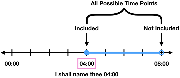
The first function on resample takes the data point from the first valid time sample. This would return the number 04:00 as the time point and the data point would belong to either 04:00 or something larger than 04:00 if it was not a given data point.
Similarly the right time and data point were obtained using resample and the resample last function. The label was to be the right number of the four hour sample bin and the interval would be closed on the right number.
df_R=df.resample('4H',label='right',closed='right').last()
df_R = df_R.rename(columns={'Date':'Left_Date','Number':'Left_Number'})
For example, the time interval from 00:00 to 04:00 would be represented by 04:00 (the right number) and the interval of time values would be from (00:00,04:00].
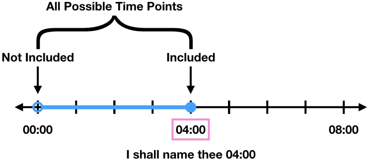
The last function on resample takes the data point from the last valid time sample. This would return the number 04:00 as the time point and the data point would belong to either 04:00 or something smaller than 04:00 if it was not a given data point.
Notice in the two figures above, if the time point 04:00 has a data value than it will be selected as both the right and left number. When this happens the weights are set to be equal (\(w_l=w_r=1/2\)). Combining the right and left points into a dataframe gives
| Left_Number | Left_Date | Right_Number | Right_Date | |
|---|---|---|---|---|
| DATE_AND_TIME | ||||
| 2017-02-18 00:00:00 | NaN | NaT | 6240218.0 | 2017-02-18 03:00:00 |
| 2017-02-18 04:00:00 | 6240218.0 | 2017-02-18 03:00:00 | 6240237.0 | 2017-02-18 07:00:00 |
| 2017-02-18 08:00:00 | 6240237.0 | 2017-02-18 07:00:00 | 6240273.0 | 2017-02-18 11:00:00 |
| 2017-02-18 12:00:00 | 6240273.0 | 2017-02-18 11:00:00 | 6240409.0 | 2017-02-18 15:00:00 |
| 2017-02-18 16:00:00 | 6240409.0 | 2017-02-18 15:00:00 | 6240650.0 | 2017-02-18 19:00:00 |
After finding the data points and times, the differences and weights were calculated.
df['Difference'] = (df['Right_Date']-df['Left_Date'])/ np.timedelta64(1, 'h')
df['Right_Differenece'] = (df['Right_Date']-df.index.values)/ np.timedelta64(1, 'h')
df['Left_Difference'] = (df.index.values-df['Left_Date'])/ np.timedelta64(1, 'h')

def get_weights(x,y):
    if y != 0:
        return x/y
    else:
        return 1/2

# Add weights needed for the weighted average to table
df['Left_Weights'] = df.apply(lambda x: get_weights(x['Right_Differenece'], x['Difference']), axis=1)
df['Right_Weights'] = df.apply(lambda x: get_weights(x['Left_Difference'], x['Difference']), axis=1)
| Left_Number | Left_Date | Right_Number | Right_Date | Difference | Right_Differenece | Left_Difference | Left_Weights | Right_Weights | |
|---|---|---|---|---|---|---|---|---|---|
| DATE_AND_TIME | |||||||||
| 2017-02-18 00:00:00 | NaN | NaT | 6240218.0 | 2017-02-18 03:00:00 | NaN | 3.0 | NaN | NaN | NaN |
| 2017-02-18 04:00:00 | 6240218.0 | 2017-02-18 03:00:00 | 6240237.0 | 2017-02-18 07:00:00 | 4.0 | 3.0 | 1.0 | 0.75 | 0.25 |
| 2017-02-18 08:00:00 | 6240237.0 | 2017-02-18 07:00:00 | 6240273.0 | 2017-02-18 11:00:00 | 4.0 | 3.0 | 1.0 | 0.75 | 0.25 |
| 2017-02-18 12:00:00 | 6240273.0 | 2017-02-18 11:00:00 | 6240409.0 | 2017-02-18 15:00:00 | 4.0 | 3.0 | 1.0 | 0.75 | 0.25 |
| 2017-02-18 16:00:00 | 6240409.0 | 2017-02-18 15:00:00 | 6240650.0 | 2017-02-18 19:00:00 | 4.0 | 3.0 | 1.0 | 0.75 | 0.25 |
The columns were then used to calculate the weighted average.
df['Weighted_Average'] = df['Left_Number']*df['Left_Weights']+df['Right_Number']*df['Right_Weights']

df = df['Weighted_Average']
| DATE_AND_TIME | Weighted Average |
|---|---|
| 2017-02-18 00:00:00 | NaN |
| 2017-02-18 04:00:00 | 6240222.75 |
| 2017-02-18 08:00:00 | 6240246.00 |
| 2017-02-18 12:00:00 | 6240307.00 |
| 2017-02-18 16:00:00 | 6240469.25 |
Final Clean Up
Having individual data for each turnstile could be interesting, but for our purposes it is better to obtain a total output for each station. To find the total output for each station summing the data seems like the obvious choice, but there are outliers and to contend with. The standard method would be to use the 1.5×IQR to define our ‘normal’ observations, replace the ‘non-normal’ observations with the mean or median of the remaining values, and then sum the total number of entries and exits. However, we are assuming each turnstile in a station has an approximately equal output, so a simple approach is to take the median (which is unaffected by outliers) and multiply it by the number of turnstiles in the station.
The final results is a data set with evenly spread time points and an approximate value for the total traffic at each station.
| DATE AND TIME | STATION | TOTAL TRAFFIC | |
|---|---|---|---|
| 0 | 02/25/2017 04:00:00 | 59 ST | 0.00 |
| 1 | 02/25/2017 08:00:00 | 59 ST | 4757.00 |
| 2 | 02/25/2017 12:00:00 | 59 ST | 13340.75 |
| 3 | 02/25/2017 16:00:00 | 59 ST | 18878.00 |
| 4 | 02/25/2017 20:00:00 | 59 ST | 18443.00 |