Introduction
Metis Bootcamp Project 1
Collaborators: Dean Miao, Derek Shi and Joseph Hamilton.
This will be the first of several Metis Bootcamp projects.
The Problem
WomenTechWomenYes was hosting their annual gala at the beginning of summer and wished to increase the number of attendees (and possible donors) by standing outside of New York City Subway Stations and letting people sign-up to collect free gala tickets through email.
Two Approaches
Our goal for the project was to find the stations with the highest traffic data from the MTA website. While the data was easy to obtain, it contained a significant amount of errors. In a previous [blog post] (https://kendallgillies.github.io/blog/Benson-Blog-WA/) I introduced the data set and a weighted average approach to cleaning the data. The weighted average approach was one of the two ways my group and I discussed cleaning the data. The other way was to use linear interpolation to find the missing data points.
When comparing linear interpolation to the weight average approach there are several things to note. Linear interpolation is itself a weighted average method. As I began to work on this blog post, I found the weights I had selected for the weighted average method were the same weights used in the linear interpolation method. A simple proof shows this. This is an important lesson in needing to truly understand the methods you are using. While I knew linear interpolation is a weighted average method, I assumed it was different from the one I was using. The code introduced in the weighted average blog post will still work for different weights.
The Data
Introduction
When first obtaining the data set from the MTA website the following variables are given:
| Variable | Description |
|---|---|
| C/A | Control Area name/Booth name. This is the internal identification of a booth at a given station. |
| UNIT | Remote unit ID of station |
| SCP | Subunit/Channel/position represents a specific address for a given terminal in each unit. |
| STATION | Subway Station name. |
| LINENAME | Train lines stopping at this location. |
| DIVISION | Represents the Line originally the station belonged to. |
| DATE | Represents the date of the audit data (MM/DD/YYYY). |
| TIME | Represents the time of the reported data (HH:MM:SS). |
| DESC | Represents the if scheduled audit event went normally. |
| ENTRIES | The cumulative entry register value for a device. |
| EXITS | The cumulative exits register value for a device. |
Using a pandas dataframe we can see an example of the output of the table.
| C/A | UNIT | SCP | STATION | LINENAME | DIVISION | DATE | TIME | DESC | ENTRIES | EXITS | |
|---|---|---|---|---|---|---|---|---|---|---|---|
| 0 | A002 | R051 | 02-00-00 | 59 ST | NQR456W | BMT | 02/18/2017 | 03:00:00 | REGULAR | 6055520 | 2052786 |
| 1 | A002 | R051 | 02-00-00 | 59 ST | NQR456W | BMT | 02/18/2017 | 07:00:00 | REGULAR | 6055537 | 2052800 |
| 2 | A002 | R051 | 02-00-00 | 59 ST | NQR456W | BMT | 02/18/2017 | 11:00:00 | REGULAR | 6055600 | 2052891 |
| 3 | A002 | R051 | 02-00-00 | 59 ST | NQR456W | BMT | 02/18/2017 | 15:00:00 | REGULAR | 6055822 | 2052960 |
| 4 | A002 | R051 | 02-00-00 | 59 ST | NQR456W | BMT | 02/18/2017 | 19:00:00 | REGULAR | 6056158 | 2053035 |
For the reasons explained in the weighed average approach post the number of features can be reduced to UNIT_AND_SCP, STATION, DATE_AND_TIME, ENTRIES and EXITS, where UNIT_AND_SCP represents the individual turnstiles for a given station and DATE_AND_TIME is a combined date and time points.
Once narrowing down to only the necessary variables, the data was separated by individual station entries and individual station exits. This information will be placed in a dictionary where the key is a combination of the station name and if the data points are for entries or exits and the value is a dataframe with the date and time variable for the index values, and the columns holding the cumulative data for either the entries or exits for each turnstile. For example, the following table is a part of the table for key 59 ST ENTRIES.
| UNIT_AND_SCP | R050 00-00-00 | R050 00-00-01 | R050 00-00-02 | R050 00-00-03 | … |
|---|---|---|---|---|---|
| DATE_AND_TIME | |||||
| 2017-02-18 03:00:00 | 6240218.0 | 8456367.0 | 2810319.0 | 52911.0 | … |
| 2017-02-18 07:00:00 | 6240237.0 | 8456370.0 | 2810321.0 | 52912.0 | … |
| 2017-02-18 11:00:00 | 6240273.0 | 8456398.0 | 2810328.0 | 52917.0 | … |
| 2017-02-18 15:00:00 | 6240409.0 | 8456484.0 | 2810371.0 | 52929.0 | … |
| 2017-02-18 19:00:00 | 6240650.0 | 8456654.0 | 2810441.0 | 52954.0 | … |
Linear Interpolation
Theoretically, each individual turnstile in each station recorded a cumulative count for entries and exits for every four hours starting at time 00:00 (midnight); however, in practice, approximately 52% of the data set contains times that did not fall on these time points. For each time point that does not fall on the desired time points there will be data for a time that is earlier (left time) and later (right time) than this time. For example, if there is not a data point for 08:00 but there are data points at 05:00 and 09:00.
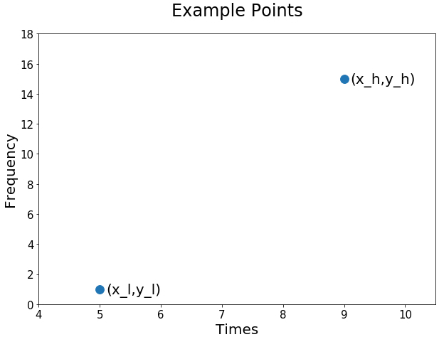
At 05:00 we will assume a data point of 1 and at 09:00 we will assume a data point of \(15\). Using the high lower notation introduced in the previous blog the example points can be labeled as follows: \(x_l = 5\), \(y_l = 1\), \(x_h = 9\) and \(y_h = 15 \). First consider a simple plot of \((x_l,y_l)=(5,1)\) and \((x_h,y_h)=(9,15)\).
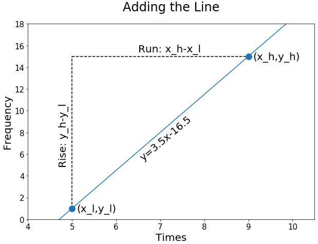
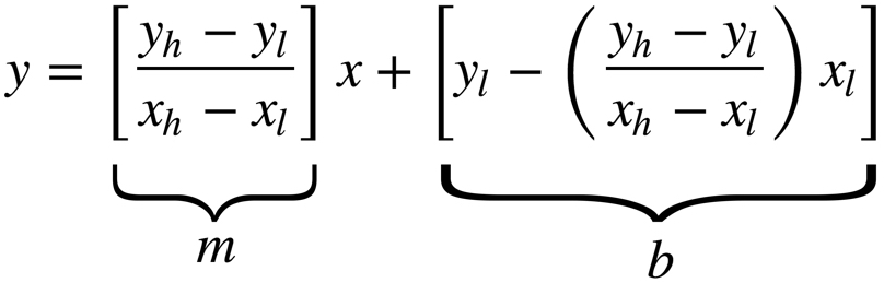
Lines take the form
where \(m\) and \(b\) denote the slope and y intercept, respectively. The line connecting the two points in our example is given by the following slope:
To find the y-intercept intercept, plug in a point and solve the equation for b.
Plugging in the slope and y-intercept, we now have the following equation for our line:
For the time point 08:00, the interpolation line gives
giving the point (8,11.5).
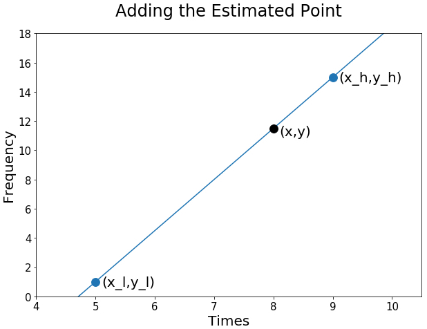
Now consider the formula for the weighted average discussed in the previous blog post. In this post our \(y_l\) and \(y_h\) are the same as \(c_l\) and \(c_h\), respectively. Notice the weighted average and the linear interpolation yield the same number.
Proof
As I previously stated, we know linear interpolation is a form of a weighted average method. To show this I will manipulate the equation for the linear interpolation line into the weighted average form
where \(w_l\) and \(w_h\) are the weights for the higher and lower points, respectively.
First consider the equation of a line,
We know the slope for linear interpolation is given by
and the y-intercept can be found by solving
for \(b\),
Plugging the slope and y-intercept into we have
Pulling out \(1/(x_h-x_l)\) gives
Distributing the information inside the brackets gives
After further simplification
Grouping the \(y_h\) and \(y_l\) terms gives
Redistributing \(1/(x_h-x_l)\) gives
which is the equation for the weighted average.
The code
Finding the weighted average using the resampling method introduced in the Weighted Average post is still usable for other weighted averages; however, using the resampling method with linear interpolation will prove to be computationally faster for our weighted average.
The python code for this is relatively simple, since pandas does all of the heavy lifting for us. Recall the data for the entries and exits for each station looks as follows.
| UNIT_AND_SCP | R050 00-00-00 | R050 00-00-01 | R050 00-00-02 | R050 00-00-03 | … |
|---|---|---|---|---|---|
| DATE_AND_TIME | |||||
| 2017-02-18 03:00:00 | 6240218.0 | 8456367.0 | 2810319.0 | 52911.0 | … |
| 2017-02-18 07:00:00 | 6240237.0 | 8456370.0 | 2810321.0 | 52912.0 | … |
| 2017-02-18 11:00:00 | 6240273.0 | 8456398.0 | 2810328.0 | 52917.0 | … |
| 2017-02-18 15:00:00 | 6240409.0 | 8456484.0 | 2810371.0 | 52929.0 | … |
| 2017-02-18 19:00:00 | 6240650.0 | 8456654.0 | 2810441.0 | 52954.0 | … |
The first step is to use interpolation to break the data up into one hour intervals.
df = df.resample('1H').interpolate()
| UNIT_AND_SCP | R050 00-00-00 | R050 00-00-01 | R050 00-00-02 | R050 00-00-03 | … |
|---|---|---|---|---|---|
| DATE_AND_TIME | |||||
| 2017-02-18 03:00:00 | 6240218.00 | 8456367.00 | 2810319.0 | 52911.00 | … |
| 2017-02-18 04:00:00 | 6240222.75 | 8456367.75 | 2810319.5 | 52911.25 | … |
| 2017-02-18 05:00:00 | 6240227.50 | 8456368.50 | 2810320.0 | 52911.50 | … |
| 2017-02-18 06:00:00 | 6240232.25 | 8456369.25 | 2810320.5 | 52911.75 | … |
| 2017-02-18 07:00:00 | 6240237.00 | 8456370.00 | 2810321.0 | 52912.00 | … |
Now that each of the hours has a representative data point, we will collapse the hours into four hour time bins and take the first possible data point on that interval for the representative data point.
df = df.resample('4H').first()
| UNIT_AND_SCP | R050 00-00-00 | R050 00-00-01 | R050 00-00-02 | R050 00-00-03 | … |
|---|---|---|---|---|---|
| DATE_AND_TIME | |||||
| 2017-02-18 00:00:00 | 6240218.00 | 8456367.00 | 2810319.00 | 52911.00 | … |
| 2017-02-18 04:00:00 | 6240222.75 | 8456367.75 | 2810319.50 | 52911.25 | … |
| 2017-02-18 08:00:00 | 6240246.00 | 8456377.00 | 2810322.75 | 52913.25 | … |
| 2017-02-18 12:00:00 | 6240307.00 | 8456419.50 | 2810338.75 | 52920.00 | … |
| 2017-02-18 16:00:00 | 6240469.25 | 8456526.50 | 2810388.50 | 52935.25 | … |
The results are the same as the weighted average method used in the weighted average post.
To compare the speed of the two methods, I took entries data for one turnstile column from the 59 ST station. The weighted average method introduced in the previous blog post took an average of 5.29 seconds to run, while the interpolation method introduced above took an average of 115 ms.
Conclusion
To recap, linear interpolation is a form of a weighted average. More specifically, it is the weighted average with the weights that are inversely related to the distance from the desired point.
The big take away from this is to always know how your methods are connected, if there is a connection. By doing a five minute mathematical proof of the two methods, I could have saved myself a lot of time and provided more useful results to the project.